Examples
These examples demonstrate most of the functionality of the package, its typical usage, and how to make some plots you might want to use.
The examples:
- The Ising Model shows how to use the package to explore the autologistic probability distribution, without concern about covariates or parameter estimation.
- Clustered Binary Data (Small $n$) shows how to use the package for regression analysis when the graph is small enough to permit computation of the normalizing constant. In this case standard maximum likelihood methods of inference can be used.
- Spatial Binary Regression shows how to use the package for autologistic regression analysis for larger, spatially-referenced graphs. In this case pseudolikelihood is used for estimation, and a (possibly parallelized) parametric bootstrap is used for inference.
The Ising Model
The term "Ising model" is usually used to refer to a Markov random field of dichotomous random variables on a regular lattice. The graph is such that each variable shares an edge only with its nearest neighbors in each dimension. It's a traditional model for magnetic spins, where the coding $(-1,1)$ is usually used. There's one parameter per vertex (a "local magnetic field") that increases or decreases the chance of getting a $+1$ state at that vertex; and there's a single pairwise parameter that controls the strength of interaction between neighbor states.
In our terminology it's just an autologistic model with the appropriate graph. Specifically, it's an ALsimple model: one with FullUnary type unary parameter, and SimplePairwise type pairwise parameter.
We can create such a model once we have the graph. For example, let's create the model on a 30-by-30 lattice:
using Autologistic, Random
Random.seed!(8888)
n = 30
G = makegrid4(n, n, (-1,1), (-1,1))
α = randn(n^2)
M1 = ALsimple(G.G, α)Above, the line G = makegrid4(n, n, (-1,1), (-1,1)) produces an n-by-n graph with vertices positioned over the square extending from $-1$ to $1$ in both directions. It returns a tuple; G.G is the graph, and G.locs is an array of tuples giving the spatial coordinates of each vertex.
M1 = ALsimple(G.G, α) creates the model. The unary parameters α were intialized to Gaussian white noise. By default the pairwise parameter is set to zero, which implies independence of the variables.
Typing M1 at the REPL shows information about the model. It's an ALsimple type with one observation of length 900.
julia> M1Autologistic model of type ALsimple with parameter vector [α; λ]. Fields: responses 900×1 Bool array unary 900×1 FullUnary with fields: α 900×1 array (unary parameter values) pairwise 900×900×1 SimplePairwise with fields: λ [0.0] (association parameter) G the graph (900 vertices, 1740 edges) count 1 (the number of observations) A 900×900 SparseMatrixCSC (the adjacency matrix) centering none coding (-1, 1) labels ("low", "high") coordinates 900-element vector of Tuple{Float64, Float64}
The conditionalprobabilities function returns the probablity of observing a $+1$ state at each vertex, conditional on the vertex's neighbor values. These can be visualized as an image, using a heatmap (from Plots.jl):
using Plots
condprobs = conditionalprobabilities(M1)
hm = heatmap(reshape(condprobs, n, n), c=:grays, aspect_ratio=1,
title="probability of +1 under independence")
plot(hm)Since the association parameter is zero, there are no neighborhood effects. The above conditional probabilities are equal to the marginal probabilities.
Next, set the association parameters to 0.75, a fairly strong association level, to introduce a neighbor effect.
setpairwiseparameters!(M1, [0.75])We can also generalize the Ising model by allowing the pairwise parameters to be different for each edge of the graph. The ALfull type represents such a model, which has a FullUnary type unary parameter, and a FullPairwise type pairwise parameter. For this example, let each edge's pairwise parameter be equal to the average distance of its two vertices from the origin.
using LinearAlgebra, Graphs
λ = [norm((G.locs[e.src] .+ G.locs[e.dst])./2) for e in edges(G.G)]
M2 = ALfull(G.G, α, λ)Autologistic model of type ALfull with parameter vector [α; Λ].
Fields:
responses 900×1 Bool array
unary 900×1 FullUnary with fields:
α 900×1 array (unary parameter values)
pairwise 900×900×1 FullPairwise with fields:
λ edge-ordered vector of association parameter values
G the graph (900 vertices, 1740 edges)
count 1 (the number of observations)
Λ 900×900 SparseMatrixCSC (the association matrix)
centering none
coding (-1, 1)
labels ("low", "high")
coordinates 900-element vector of Tuple{Float64, Float64}
A quick way to compare models with nonzero association is to observe random samples from the models. The sample function can be used to do this. For this example, use perfect sampling using a bounding chain algorithm.
s1 = sample(M1, method=perfect_bounding_chain)
s2 = sample(M2, method=perfect_bounding_chain)Other options are available for sampling. The enumeration SamplingMethods lists them. The samples we have just drawn can also be visualized using heatmap:
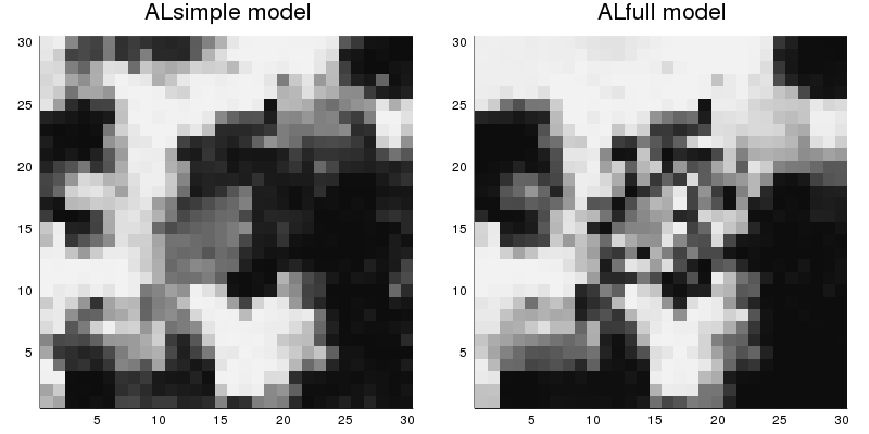
pl1 = heatmap(reshape(s1, n, n), c=:grays, colorbar=false, title="ALsimple model");
pl2 = heatmap(reshape(s2, n, n), c=:grays, colorbar=false, title="ALfull model");
plot(pl1, pl2, size=(800,400), aspect_ratio=1)In these plots, black indicates the low state, and white the high state. A lot of local clustering is occurring in the samples due to the neighbor effects. For the ALfull model, clustering is greater farther from the center of the square.
To see the long-run differences between the two models, we can look at the marginal probabilities. They can be estimated by drawing many samples and averaging them (note that running this code chunk can take a few minutes):
marg1 = sample(M1, 500, method=perfect_bounding_chain, verbose=true, average=true)
marg2 = sample(M2, 500, method=perfect_bounding_chain, verbose=true, average=true)
pl3 = heatmap(reshape(marg1, n, n), c=:grays,
colorbar=false, title="ALsimple model");
pl4 = heatmap(reshape(marg2, n, n), c=:grays,
colorbar=false, title="ALfull model");
plot(pl3, pl4, size=(800,400), aspect_ratio=1)
savefig("marginal-probs.png")The figure marginal-probs.png looks like this:
The differences between the two marginal distributions are due to the different association structures, because the unary parts of the two models are the same. The ALfull model has stronger association near the edges of the square, and weaker association near the center. The ALsimple model has a moderate association level throughout.
As a final demonstration, perform Gibbs sampling for model M2, starting from a random state. Display a gif animation of the progress.
nframes = 150
gibbs_steps = sample(M2, nframes, method=Gibbs)
anim = @animate for i = 1:nframes
heatmap(reshape(gibbs_steps[:,i], n, n), c=:grays, colorbar=false,
aspect_ratio=1, title="Gibbs sampling: step $(i)")
end
gif(anim, "ising_gif.gif", fps=10)
Clustered Binary Data (Small $n$)
The retinitis pigmentosa data set (obtained from this source) is an opthalmology data set. The data comes from 444 patients that had both eyes examined. The data can be loaded with Autologistic.datasets:
julia> using Autologistic, DataFrames, Graphsjulia> df = Autologistic.datasets("pigmentosa");julia> first(df, 6)6×9 DataFrame Row │ ID aut_dom aut_rec sex_link age sex psc eye va │ Int64 Int64 Int64 Int64 Int64 Int64 Int64 Int64 Int64 ─────┼────────────────────────────────────────────────────────────────────── 1 │ 7 0 0 0 27 0 1 0 0 2 │ 7 0 0 0 27 0 1 1 1 3 │ 8 0 1 0 44 1 0 0 0 4 │ 8 0 1 0 44 1 0 1 0 5 │ 19 0 0 0 24 0 1 0 1 6 │ 19 0 0 0 24 0 1 1 1julia> describe(df)9×7 DataFrame Row │ variable mean min median max nmissing eltype │ Symbol Float64 Int64 Float64 Int64 Int64 DataType ─────┼─────────────────────────────────────────────────────────────────── 1 │ ID 1569.22 7 1466.5 3392 0 Int64 2 │ aut_dom 0.0990991 0 0.0 1 0 Int64 3 │ aut_rec 0.141892 0 0.0 1 0 Int64 4 │ sex_link 0.0608108 0 0.0 1 0 Int64 5 │ age 34.2342 6 32.5 80 0 Int64 6 │ sex 0.576577 0 1.0 1 0 Int64 7 │ psc 0.432432 0 0.0 1 0 Int64 8 │ eye 0.5 0 0.5 1 0 Int64 9 │ va 0.504505 0 1.0 1 0 Int64
The response for each eye is va, an indicator of poor visual acuity (coded 0 = no, 1 = yes in the data set). Seven covariates were also recorded for each eye:
- aut_dom: autosomal dominant (0=no, 1=yes)
- aut_rec: autosomal recessive (0=no, 1=yes)
- sex_link: sex-linked (0=no, 1=yes)
- age: age (years, range 6-80)
- sex: gender (0=female, 1=male)
- psc: posterior subscapsular cataract (0=no, 1=yes)
- eye: which eye is it? (0=left, 1=right)
The last four factors are relevant clinical observations, and the first three are genetic factors. The data set also includes an ID column with an ID number specific to each patient. Eyes with the same ID come from the same person.
The natural unit of analysis is the eye, but pairs of observations from the same patient are "clustered" because the occurrence of acuity loss in the left and right eye is probably correlated. We can model each person's two va outcomes as two dichotomous random variables with a 2-vertex, 1-edge graph.
julia> G = Graph(2,1){2, 1} undirected simple Int64 graph
Each of the 444 bivariate observations has this graph, and each has its own set of covariates.
If we include all seven predictors, plus intercept, in our model, we have 2 variables per observation, 8 predictors, and 444 observations.
Before creating the model we need to re-structure the covariates. The data in df has one row per eye, with the variable ID indicating which eyes belong to the same patient. We need to rearrange the responses (Y) and the predictors (X) into arrays suitable for our autologistic models, namely:
Yis $2 \times 444$ with one observation per column.Xis $2 \times 8 \times 444$ with one $2 \times 8$ matrix of predictors for each observation. The first column of each predictor matrix is an intercept column, and columns 2 through 8 are foraut_dom,aut_rec,sex_link,age,sex,psc, andeye, respectively.
X = Array{Float64,3}(undef, 2, 8, 444);
Y = Array{Float64,2}(undef, 2, 444);
for i in 1:2:888
patient = Int((i+1)/2)
X[1,:,patient] = [1 permutedims(Vector(df[i,2:8]))]
X[2,:,patient] = [1 permutedims(Vector(df[i+1,2:8]))]
Y[:,patient] = convert(Array, df[i:i+1, 9])
endFor example, patient 100 had responses
julia> Y[:,100]2-element Vector{Float64}: 1.0 0.0
Indicating visual acuity loss in the left eye, but not in the right. The predictors for this individual are
julia> X[:,:,100]2×8 Matrix{Float64}: 1.0 0.0 0.0 0.0 18.0 1.0 1.0 0.0 1.0 0.0 0.0 0.0 18.0 1.0 1.0 1.0
Now we can create our autologistic regression model.
model = ALRsimple(G, X, Y=Y)Autologistic regression model of type ALRsimple with parameter vector [β; λ].
Fields:
responses 2×444 Bool array
unary 2×444 LinPredUnary with fields:
X 2×8×444 array (covariates)
β 8-element vector (regression coefficients)
pairwise 2×2×444 SimplePairwise with fields:
λ [0.0] (association parameter)
G the graph (2 vertices, 1 edges)
count 444 (the number of observations)
A 2×2 SparseMatrixCSC (the adjacency matrix)
centering none
coding (-1, 1)
labels ("low", "high")
coordinates 2-element vector of Tuple{Float64, Float64}
This creates a model with the "simple pairwise" structure, using a single association parameter. The default is to use no centering adjustment, and to use coding $(-1,1)$ for the responses. This "symmetric" version of the model is recommended for a variety of reasons. Using different coding or centering choices is only recommended if you have a thorough understanding of what you are doing; but if you wish to use different choices, this can easily be done using keyword arguments. For example, ALRsimple(G, X, Y=Y, coding=(0,1), centering=expectation) creates the "centered autologistic model" that has appeared in the literature (e.g., here and here).
The model has nine parameters (eight regression coefficients plus the association parameter). All parameters are initialized to zero:
julia> getparameters(model)9-element Vector{Float64}: 0.0 0.0 0.0 0.0 0.0 0.0 0.0 0.0 0.0
When we call getparameters, the vector returned always has the unary parameters first, with the pairwise parameter(s) appended at the end.
Because there are only two vertices in the graph, we can use the full likelihood (fit_ml! function) to do parameter estimation. This function returns a structure with the estimates as well as standard errors, p-values, and 95% confidence intervals for the parameter estimates.
out = fit_ml!(model)Autologistic model fitting results. Its non-empty fields are:
estimate 9-element vector of parameter estimates
se 9-element vector of standard errors
pvalues 9-element vector of 2-sided p-values
CIs 9-element vector of 95% confidence intervals (as tuples)
optim the output of the call to optimize()
Hinv the inverse of the Hessian, evaluated at the optimum
kwargs extra keyword arguments passed to sample()
convergence true
Use summary(fit; [parnames, sigdigits]) to see a table of estimates.
For pseudolikelihood, use oneboot() and addboot!() to add bootstrap after the fact.To view the estimation results, use summary:
summary(out, parnames = ["icept", "aut_dom", "aut_rec", "sex_link", "age", "sex",
"psc", "eye", "λ"])name est se p-value 95% CI
icept -0.264 0.0973 0.00668 (-0.455, -0.0732)
aut_dom -0.167 0.0932 0.0734 (-0.349, 0.0158)
aut_rec 0.104 0.0787 0.188 (-0.0507, 0.258)
sex_link 0.301 0.126 0.0168 (0.0542, 0.547)
age 0.00492 0.00184 0.00763 (0.00131, 0.00853)
sex 0.0207 0.0557 0.711 (-0.0885, 0.13)
psc 0.139 0.0589 0.0185 (0.0233, 0.254)
eye 0.0273 0.12 0.819 (-0.207, 0.262)
λ 0.818 0.0656 0.0 (0.69, 0.947)From this we see that the association parameter is fairly large (0.818), supporting the idea that the left and right eyes are associated. It is also highly statistically significant. Among the covariates, sex_link, age, and psc are all statistically significant.
Spatial Binary Regression
ALR models are natural candidates for analysis of spatial binary data, where locations in the same neighborhood are more likely to have the same outcome than sites that are far apart. The hydrocotyle data provide a typical example. The response in this data set is the presence/absence of a certain plant species in a grid of 2995 regions covering Germany. The data set is included in Autologistic.jl:
julia> using Autologistic, DataFrames, Graphsjulia> df = Autologistic.datasets("hydrocotyle")2995×5 DataFrame Row │ X Y altitude temperature obs │ Int64 Int64 Float64 Float64 Int64 ──────┼──────────────────────────────────────────── 1 │ 16 1 1.71139 8.2665 1 2 │ 15 2 1.8602 8.15482 1 3 │ 16 2 1.7858 8.09898 1 4 │ 17 2 1.7858 8.09898 0 5 │ 18 2 1.7858 8.09898 0 6 │ 19 2 1.8602 8.09898 1 7 │ 15 3 1.8602 8.15482 1 8 │ 16 3 1.7858 8.15482 1 ⋮ │ ⋮ ⋮ ⋮ ⋮ ⋮ 2989 │ 26 78 16.4442 2.6269 0 2990 │ 27 78 15.3281 3.5203 0 2991 │ 28 78 17.6347 1.90102 0 2992 │ 31 78 16.3698 -0.5 0 2993 │ 32 78 15.4025 -0.5 0 2994 │ 33 78 16.3698 0.281726 0 2995 │ 27 79 18.23 1.95685 0 2980 rows omitted
In the data frame, the variables X and Y give the spatial coordinates of each region (in dimensionless integer units), obs gives the presence/absence data (1 = presence), and altitude and temperature are covariates.
We will use an ALRsimple model for these data. The graph can be formed using makespatialgraph:
locations = [(df.X[i], df.Y[i]) for i in 1:size(df,1)]
g = makespatialgraph(locations, 1.0)makespatialgraph creates the graph by adding edges between any vertices with Euclidean distance smaller than a cutoff distance (Graphs.jl has a euclidean_graph function that does the same thing). For these data arranged on a grid, a threshold of 1.0 will make a 4-nearest-neighbors lattice. Letting the threshold be sqrt(2) would make an 8-nearest-neighbors lattice.
We can visualize the graph, the responses, and the predictors using GraphRecipes.jl (there are several other options for plotting graphs as well).
using GraphRecipes, Plots
# Function to convert a value to a gray shade
makegray(x, lo, hi) = RGB([(x-lo)/(hi-lo) for i=1:3]...)
# Function to plot the graph with node shading determined by v.
# Plot each node as a square and don't show the edges.
function myplot(v, lohi=nothing)
colors = lohi==nothing ? makegray.(v, minimum(v), maximum(v)) : makegray.(v, lohi[1], lohi[2])
return graphplot(g.G, x=df.X, y=df.Y, background_color = :lightblue,
marker = :square, markersize=2, markerstrokewidth=0,
markercolor = colors, yflip = true, linecolor=nothing)
end
# Make the plot
plot(myplot(df.obs), myplot(df.altitude), myplot(df.temperature),
layout=(1,3), size=(800,300), titlefontsize=8,
title=hcat("Species Presence (white = yes)", "Altitude (lighter = higher)",
"Temperature (lighter = higher)"))Constructing the model
We can see that the species primarily is found at low-altitude locations. To model the effect of altitude and temperature on species presence, construct an ALRsimple model.
# Autologistic.jl reqiures predictors to be a matrix of Float64
Xmatrix = Array{Float64}([ones(2995) df.altitude df.temperature])
# Create the model
hydro = ALRsimple(g.G, Xmatrix, Y=df.obs)Autologistic regression model of type ALRsimple with parameter vector [β; λ].
Fields:
responses 2995×1 Bool array
unary 2995×1 LinPredUnary with fields:
X 2995×3×1 array (covariates)
β 3-element vector (regression coefficients)
pairwise 2995×2995×1 SimplePairwise with fields:
λ [0.0] (association parameter)
G the graph (2995 vertices, 5804 edges)
count 1 (the number of observations)
A 2995×2995 SparseMatrixCSC (the adjacency matrix)
centering none
coding (-1, 1)
labels ("low", "high")
coordinates 2995-element vector of Tuple{Float64, Float64}
The model hydro has four parameters: three regression coefficients (interceept, altitude, and temperature) plus an association parameter. It is a "symmetric" autologistic model, because it has a coding symmetric around zero and no centering term.
Fitting the model by pseudolikelihood
With 2995 nodes in the graph, the likelihood is intractable for this case. Use fit_pl! to do parameter estimation by pseudolikelihood instead. The fitting function uses the BFGS algorithm via Optim.jl. Any of Optim's general options can be passed to fit_pl! to control the optimization. We have found that allow_f_increases often aids convergence. It is used here:
julia> fit1 = fit_pl!(hydro, allow_f_increases=true)Autologistic model fitting results. Its non-empty fields are: estimate 4-element vector of parameter estimates optim the output of the call to optimize() kwargs extra keyword arguments passed to sample() convergence true Use summary(fit; [parnames, sigdigits]) to see a table of estimates. For pseudolikelihood, use oneboot() and addboot!() to add bootstrap after the fact.julia> parnames = ["intercept", "altitude", "temperature", "association"];julia> summary(fit1, parnames=parnames)name est se p-value 95% CI intercept -0.192 altitude -0.0573 temperature 0.0498 association 0.361
fit_pl! mutates the model object by setting its parameters to the optimal values. It also returns an object, of type ALfit, which holds information about the result. Calling summary(fit1) produces a summary table of the estimates. For now there are no standard errors. This will be addressed below.
To quickly visualize the quality of the fitted model, we can use sampling to get the marginal probabilities, and to observe specific samples.
# Average 500 samples to estimate marginal probability of species presence
marginal1 = sample(hydro, 500, method=perfect_bounding_chain, average=true)
# Draw 2 random samples for visualizing generated data.
draws = sample(hydro, 2, method=perfect_bounding_chain)
# Plot them
plot(myplot(marginal1, (0,1)), myplot(draws[:,1]), myplot(draws[:,2]),
layout=(1,3), size=(800,300), titlefontsize=8,
title=["Marginal Probability" "Random sample 1" "Random Sample 2"])In the above code, perfect sampling was used to draw samples from the fitted distribution. The marginal plot shows consistency with the observed data, and the two generated data sets show a level of spatial clustering similar to the observed data.
Error estimation 1: bootstrap after the fact
A parametric bootstrap can be used to get an estimate of the precision of the estimates returned by fit_pl!. The function oneboot has been included in the package to facilitate this. Each call of oneboot draws a random sample from the fitted distribution, then re-fits the model using this sample as the responses. It returns a named tuple giving the sample, the parameter estimates, and a convergence flag. Any extra keyword arguments are passed on to sample or optimize as appropriate to control the process.
julia> # Do one bootstrap replication for demonstration purposes. oneboot(hydro, allow_f_increases=true, method=perfect_bounding_chain)(sample = [1.0, 1.0, 1.0, 1.0, 1.0, 1.0, 1.0, 1.0, 1.0, 1.0 … -1.0, -1.0, -1.0, -1.0, -1.0, -1.0, -1.0, -1.0, -1.0, -1.0], estimate = [-0.7882971346219423, -0.0544360040569443, 0.12015935739429248, 0.36594211978958097], convergence = true)
An array of the tuples produced by oneboot can be fed to addboot! to update the fitting summary with precision estimates:
nboot = 2000
boots = [oneboot(hydro, allow_f_increases=true, method=perfect_bounding_chain) for i=1:nboot]
addboot!(fit1, boots)At the time of writing, this took about 5.7 minutes on the author's workstation. After adding the bootstrap information, the fitting results look like this:
julia> summary(fit1,parnames=parnames)
name est se 95% CI
intercept -0.192 0.319 (-0.858, 0.4)
altitude -0.0573 0.015 (-0.0887, -0.0296)
temperature 0.0498 0.0361 (-0.0163, 0.126)
association 0.361 0.018 (0.326, 0.397)Confidence intervals for altitude and the association parameter both exclude zero, so we conclude that they are statistically significant.
Error estimation 2: (parallel) bootstrap when fitting
Alternatively, the bootstrap inference procedure can be done at the same time as fitting by providing the keyword argument nboot (which specifies the number of bootstrap samples to generate) when calling fit_pl!. If you do this, and you have more than one worker process available, then the bootstrap will be done in parallel across the workers (using an @distributed for loop). This makes it easy to achieve speed gains from parallelism on multicore workstations.
using Distributed # needed for parallel computing
addprocs(6) # create 6 worker processes
@everywhere using Autologistic # workers need the package loaded
fit2 = fit_pl!(hydro, nboot=2000,
allow_f_increases=true, method=perfect_bounding_chain)In this case the 2000 bootstrap replications took about 1.1 minutes on the same 6-core workstation. The output object fit2 already includes the confidence intervals:
julia> summary(fit2, parnames=parnames)
name est se 95% CI
intercept -0.192 0.33 (-0.9, 0.407)
altitude -0.0573 0.0157 (-0.0897, -0.0297)
temperature 0.0498 0.0372 (-0.0169, 0.13)
association 0.361 0.0179 (0.327, 0.396)For parallel computing of the bootstrap in other settings (eg. on a cluster), it should be fairly simple implement in a script, using the oneboot/addboot! approach of the previous section.
Comparison to logistic regression
If we ignore spatial association, and just fit the model with ordinary logistic regression, we get the following result:
using GLM
LR = glm(@formula(obs ~ altitude + temperature), df, Bernoulli(), LogitLink());
coef(LR)3-element Vector{Float64}:
5.967115773790056
-0.8273369416876384
-0.37382566103477355As mentioned in The Symmetric Model and Logistic Regression, the logistic regression coefficients are not directly comparable to the ALR coefficients, because the ALR model uses $(-1, 1)$ coding. If we want to make the parameters comparable, we can either transform the symmetric model's parameters, or fit the transformed symmetric model (a model with $(0,1)$ coding and centering=onehalf).
The parameter transformation is done as follows:
transformed_pars = [2*getunaryparameters(hydro); 4*getpairwiseparameters(hydro)]4-element Vector{Float64}:
-0.3831243912292679
-0.11460656354652317
0.09962289660191388
1.4457110224119458We see that the association parameter is large (1.45), but the regression parameters are small compared to the logistic regression model. This is typical: ignoring spatial association tends to result in overestimation of the regression effects.
We can fit the transformed model directly, to illustrate that the result is the same:
same_as_hydro = ALRsimple(g.G, Xmatrix, Y=df.obs, coding=(0,1), centering=onehalf)
fit3 = fit_pl!(same_as_hydro, allow_f_increases=true)
fit3.estimate4-element Vector{Float64}:
-0.3831243879951975
-0.11460656331406432
0.09962289610205548
1.445711022585812We see that the parameter estimates from same_as_hydro are equal to the hydro estimates after transformation.
Comparison to the centered model
The centered autologistic model can be easily constructed for comparison with the symmetric one. We can start with a copy of the symmetric model we have already created.
The pseudolikelihood function for the centered model is not convex. Three different local optima were found. For this demonstration we are using the start argument to let optimization start from a point close to the best minimum found.
centered_hydro = deepcopy(hydro)
centered_hydro.coding = (0,1)
centered_hydro.centering = expectation
fit4 = fit_pl!(centered_hydro, nboot=2000, start=[-1.7, -0.17, 0.0, 1.5],
allow_f_increases=true, method=perfect_bounding_chain)julia> summary(fit4, parnames=parnames)
name est se 95% CI
intercept -2.29 1.07 (-4.6, -0.345)
altitude -0.16 0.0429 (-0.258, -0.088)
temperature 0.0634 0.115 (-0.138, 0.32)
association 1.51 0.0505 (1.42, 1.61)
julia> round.([fit3.estimate fit4.estimate], digits=3)
4×2 Array{Float64,2}:
-0.383 -2.29
-0.115 -0.16
0.1 0.063
1.446 1.506The main difference between the symmetric ALR model and the centered one is the intercept, which changes from -0.383 to -2.29 when changing to the centered model. This is not a small difference. To see this, compare what the two models predict in the absence of spatial association.
# Change models to have association parameters equal to zero
# Remember parameters are always Array{Float64,1}.
setpairwiseparameters!(centered_hydro, [0.0])
setpairwiseparameters!(hydro, [0.0])
# Sample to estimate marginal probabilities
centered_marg = sample(centered_hydro, 500, method=perfect_bounding_chain, average=true)
symmetric_marg = sample(hydro, 500, method=perfect_bounding_chain, average=true)
# Plot to compare
plot(myplot(centered_marg, (0,1)), myplot(symmetric_marg, (0,1)),
layout=(1,2), size=(500,300), titlefontsize=8,
title=["Centered Model" "Symmetric Model"])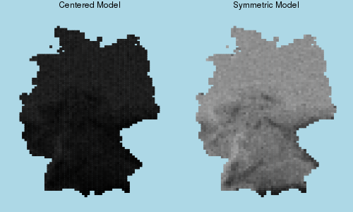
If we remove the spatial association term, the centered model predicts a very low probability of seeing the plant anywhere–including in locations with low elevation, where the plant is plentiful in reality. This is a manifestation of a problem with the centered model, where parameter interpretability is lost when association becomes strong.